This is my solution for homework 4 of 95-851 Making Products Count: Data Science for Product Management. This is a good practice for data manipulation and KMeans clustering in sklearn.
The goal of this project is to group bike shops with similar bikes sales pattern. Based on the assumption that bikes are selected by its model, price, and other features, customers may have different preferences towards bike shops. We’ll find this pattern using K means Clustering.
We are given three datasets: bikes, order, bikeshops. The first step is to merge them and aggregate bikes order for all 30 bike shops. Then, to scale the quantity, we transform the quantity to the relative quantity(percentage). Last, we choose the right number of clusters to perform K-means Clustering.
import pandas as pd
import numpy as np

import matplotlib.pyplot as plt
import seaborn as sns
Step 1: Read Datasets
bike = pd.ExcelFile("bikes.xlsx").parse("Sheet1")
shop = pd.ExcelFile("bikeshops.xlsx").parse("Sheet1")
order = pd.ExcelFile("orders.xlsx").parse("Sheet1")
order.info()
<class 'pandas.core.frame.DataFrame'>
Int64Index: 15644 entries, 1 to 15644
Data columns (total 6 columns):
order.id       15644 non-null int64
order.line     15644 non-null int64
order.date     15644 non-null datetime64[ns]
customer.id    15644 non-null int64
product.id     15644 non-null int64
quantity       15644 non-null int64
dtypes: datetime64[ns](1), int64(5)
memory usage: 855.5 KB
bike.head()
| bike.id | model | category1 | category2 | frame | price | |
|---|---|---|---|---|---|---|
| 0 | 1 | Supersix Evo Black Inc. | Road | Elite Road | Carbon | 12790 |
| 1 | 2 | Supersix Evo Hi-Mod Team | Road | Elite Road | Carbon | 10660 |
| 2 | 3 | Supersix Evo Hi-Mod Dura Ace 1 | Road | Elite Road | Carbon | 7990 |
| 3 | 4 | Supersix Evo Hi-Mod Dura Ace 2 | Road | Elite Road | Carbon | 5330 |
| 4 | 5 | Supersix Evo Hi-Mod Utegra | Road | Elite Road | Carbon | 4260 |
shop.head()
| bikeshop.id | bikeshop.name | bikeshop.city | bikeshop.state | latitude | longitude | |
|---|---|---|---|---|---|---|
| 0 | 1 | Pittsburgh Mountain Machines | Pittsburgh | PA | 40.440625 | -79.995886 |
| 1 | 2 | Ithaca Mountain Climbers | Ithaca | NY | 42.443961 | -76.501881 |
| 2 | 3 | Columbus Race Equipment | Columbus | OH | 39.961176 | -82.998794 |
| 3 | 4 | Detroit Cycles | Detroit | MI | 42.331427 | -83.045754 |
| 4 | 5 | Cincinnati Speed | Cincinnati | OH | 39.103118 | -84.512020 |
order.head()
| order.id | order.line | order.date | customer.id | product.id | quantity | |
|---|---|---|---|---|---|---|
| 1 | 1 | 1 | 2011-01-07 | 2 | 48 | 1 |
| 2 | 1 | 2 | 2011-01-07 | 2 | 52 | 1 |
| 3 | 2 | 1 | 2011-01-10 | 10 | 76 | 1 |
| 4 | 2 | 2 | 2011-01-10 | 10 | 52 | 1 |
| 5 | 3 | 1 | 2011-01-10 | 6 | 2 | 1 |
Step 2: Merge three datasets
order_shop=pd.merge(left=order, right=shop, how='outer', left_on="customer.id", right_on="bikeshop.id")
order_final = pd.merge(left=order_shop,right = bike,left_on = "product.id",right_on="bike.id")
order_final.head()
| order.id | order.line | order.date | customer.id | product.id | quantity | bikeshop.id | bikeshop.name | bikeshop.city | bikeshop.state | latitude | longitude | bike.id | model | category1 | category2 | frame | price | |
|---|---|---|---|---|---|---|---|---|---|---|---|---|---|---|---|---|---|---|
| 0 | 1 | 1 | 2011-01-07 | 2 | 48 | 1 | 2 | Ithaca Mountain Climbers | Ithaca | NY | 42.443961 | -76.501881 | 48 | Jekyll Carbon 2 | Mountain | Over Mountain | Carbon | 6070 |
| 1 | 132 | 6 | 2011-05-13 | 2 | 48 | 1 | 2 | Ithaca Mountain Climbers | Ithaca | NY | 42.443961 | -76.501881 | 48 | Jekyll Carbon 2 | Mountain | Over Mountain | Carbon | 6070 |
| 2 | 507 | 2 | 2012-06-26 | 2 | 48 | 1 | 2 | Ithaca Mountain Climbers | Ithaca | NY | 42.443961 | -76.501881 | 48 | Jekyll Carbon 2 | Mountain | Over Mountain | Carbon | 6070 |
| 3 | 528 | 18 | 2012-07-16 | 2 | 48 | 1 | 2 | Ithaca Mountain Climbers | Ithaca | NY | 42.443961 | -76.501881 | 48 | Jekyll Carbon 2 | Mountain | Over Mountain | Carbon | 6070 |
| 4 | 691 | 13 | 2013-02-05 | 2 | 48 | 1 | 2 | Ithaca Mountain Climbers | Ithaca | NY | 42.443961 | -76.501881 | 48 | Jekyll Carbon 2 | Mountain | Over Mountain | Carbon | 6070 |
Step 3: Convert Unit Price
#order_final.groupby(['model','category1','category2','frame'])['price'].median().median()
#order_final.price.median()
#order_final.groupby(['category1','category2','frame'])['price'].unique().apply(np.median)
order_final.groupby('model').price.unique().apply(lambda x:x[0]).median()
#np.sort(order_final.price.unique())
#np.sort(order_final.price.unique())
3200.0
Median Price for all the models are 3200. So we categorize price lower than and eqaul to 3200 as low, otherwise high.
#order_final["category median"]=order_final.groupby(['category1','category2','frame'])['price'].transform(lambda x:np.median(x.unique()))
#order_final['unitPrice']=(order_final['price']>order_final["category median"]).apply(lambda x: "high" if x==True else "low")
order_final['unitPrice']=order_final['price'].apply(lambda x: 'high' if x>3200 else 'low')
Step 4: Obtain pivot table
summary=order_final.groupby(['bikeshop.name', 'model', 'category1', 'category2', 'frame', 'price','unitPrice']).quantity.sum().reset_index()
customers = summary[["bikeshop.name","model","quantity"]].pivot(index="bikeshop.name",columns = "model",values="quantity").fillna(0).reset_index().rename_axis(None,1)
summary.head()
| bikeshop.name | model | category1 | category2 | frame | price | unitPrice | quantity | |
|---|---|---|---|---|---|---|---|---|
| 0 | Albuquerque Cycles | Bad Habit 1 | Mountain | Trail | Aluminum | 3200 | low | 5 |
| 1 | Albuquerque Cycles | Bad Habit 2 | Mountain | Trail | Aluminum | 2660 | low | 2 |
| 2 | Albuquerque Cycles | Beast of the East 1 | Mountain | Trail | Aluminum | 2770 | low | 3 |
| 3 | Albuquerque Cycles | Beast of the East 2 | Mountain | Trail | Aluminum | 2130 | low | 3 |
| 4 | Albuquerque Cycles | Beast of the East 3 | Mountain | Trail | Aluminum | 1620 | low | 1 |
Get ratio
scaling
customers=customers.set_index("bikeshop.name")
customers['sum']=customers.sum(axis=1)
customers=customers.div(customers["sum"], axis=0).drop('sum',axis=1)
customers.head()
| Bad Habit 1 | Bad Habit 2 | Beast of the East 1 | Beast of the East 2 | Beast of the East 3 | CAAD Disc Ultegra | CAAD12 105 | CAAD12 Black Inc | CAAD12 Disc 105 | CAAD12 Disc Dura Ace | ... | Synapse Sora | Trail 1 | Trail 2 | Trail 3 | Trail 4 | Trail 5 | Trigger Carbon 1 | Trigger Carbon 2 | Trigger Carbon 3 | Trigger Carbon 4 | |
|---|---|---|---|---|---|---|---|---|---|---|---|---|---|---|---|---|---|---|---|---|---|
| bikeshop.name | |||||||||||||||||||||
| Albuquerque Cycles | 0.017483 | 0.006993 | 0.01049 | 0.010490 | 0.003497 | 0.013986 | 0.006993 | 0.000000 | 0.013986 | 0.048951 | ... | 0.000000 | 0.000000 | 0.003497 | 0.006993 | 0.017483 | 0.010490 | 0.006993 | 0.003497 | 0.006993 | 0.006993 |
| Ann Arbor Speed | 0.006645 | 0.009967 | 0.01495 | 0.009967 | 0.003322 | 0.026578 | 0.014950 | 0.016611 | 0.014950 | 0.008306 | ... | 0.009967 | 0.009967 | 0.014950 | 0.009967 | 0.003322 | 0.011628 | 0.000000 | 0.000000 | 0.000000 | 0.011628 |
| Austin Cruisers | 0.008130 | 0.004065 | 0.00813 | 0.008130 | 0.000000 | 0.020325 | 0.020325 | 0.004065 | 0.024390 | 0.008130 | ... | 0.020325 | 0.016260 | 0.016260 | 0.016260 | 0.008130 | 0.008130 | 0.000000 | 0.000000 | 0.000000 | 0.016260 |
| Cincinnati Speed | 0.005115 | 0.000000 | 0.00000 | 0.000000 | 0.000000 | 0.015345 | 0.010230 | 0.015345 | 0.007673 | 0.017903 | ... | 0.012788 | 0.000000 | 0.002558 | 0.002558 | 0.002558 | 0.000000 | 0.010230 | 0.007673 | 0.010230 | 0.020460 |
| Columbus Race Equipment | 0.010152 | 0.000000 | 0.00000 | 0.005076 | 0.002538 | 0.010152 | 0.027919 | 0.027919 | 0.025381 | 0.012690 | ... | 0.015228 | 0.002538 | 0.002538 | 0.005076 | 0.000000 | 0.000000 | 0.010152 | 0.005076 | 0.017766 | 0.005076 |
5 rows × 97 columns
Step 5: KMeans Clustering
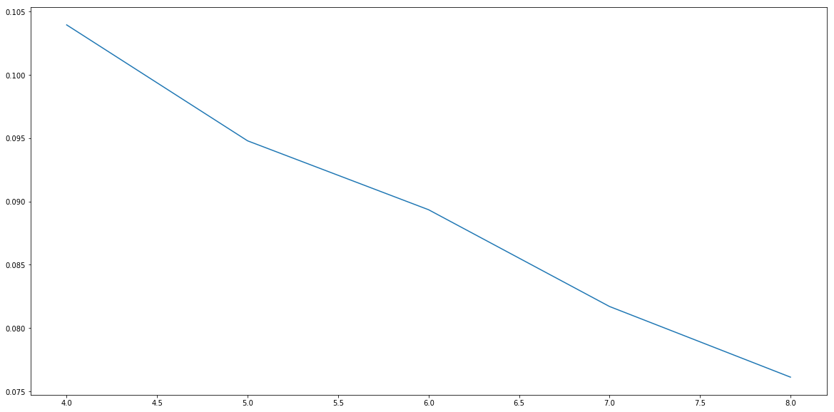
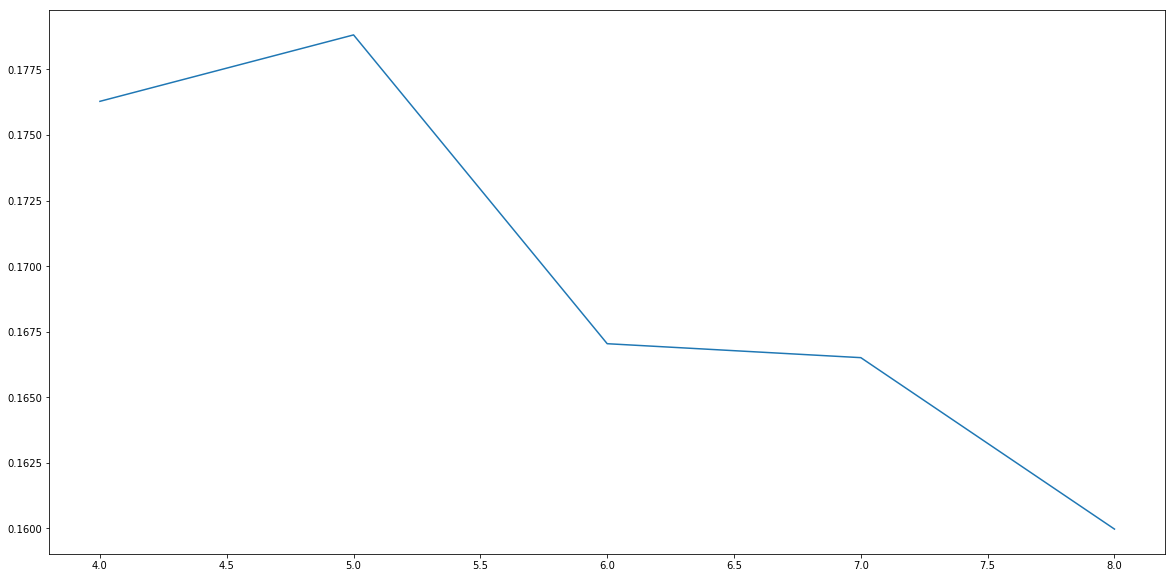
I used elbow method and silhouette analysis to determine the number of clusters. It is hard to tell from elbow method but silhouette analysis clearly suggests K=5.
from sklearn.cluster import KMeans
inertias = []
for i in range(4,9):
    kmean = KMeans(n_clusters=i,random_state=20,n_init=50)
    kmean.fit(customers)
    inertias.append(kmean.inertia_)

import matplotlib.pyplot as plt
plt.figure(figsize=(20,10))
plt.plot(range(4,9),inertias)
[<matplotlib.lines.Line2D at 0x148f94dc0b8>]

from sklearn.metrics import silhouette_samples, silhouette_score
silhouette = []
for i in range(4,9):
    clusterer = KMeans(n_clusters=i, random_state=20,n_init=50)
    cluster_labels = clusterer.fit_predict(customers)

    # The silhouette_score gives the average value for all the samples.
    # This gives a perspective into the density and separation of the formed
    # clusters
    silhouette_avg = silhouette_score(customers, cluster_labels)
    silhouette.append(silhouette_avg)
    #print("For n_clusters =",i,
    #      "The average silhouette_score is :", silhouette_avg)

import matplotlib.pyplot as plt
plt.figure(figsize=(20,10))
plt.plot(range(4,9),silhouette)
[<matplotlib.lines.Line2D at 0x148f9c42080>]

Step 6: Cluster Analysis
clusterer = KMeans(n_clusters=5, random_state=20,n_init=50)
cluster_labels = clusterer.fit_predict(customers)
customers['group'] = cluster_labels
import seaborn as sns
plt.figure(figsize=(10,10))
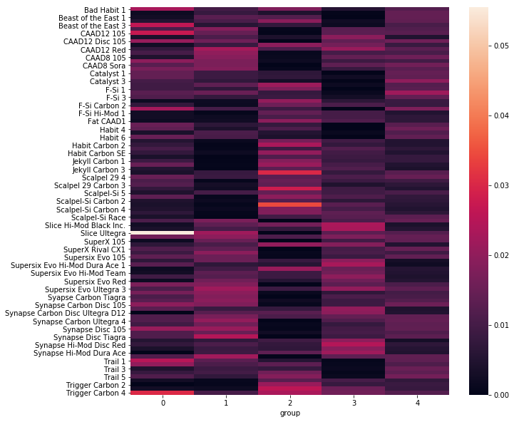
sns.heatmap(customers.groupby("group").mean().T)
#plt.figure(figsize=(10,10))
#sns.heatmap(customers.groupby("group").mean())
#customers.groupby("group").mean()
<matplotlib.axes._subplots.AxesSubplot at 0x148f5f982e8>

pd.set_option('max_colwidth', 800)
pd.DataFrame(customers.reset_index().groupby("group")["bikeshop.name"].unique())
| bikeshop.name | |
|---|---|
| group | |
| 0 | [Philadelphia Bike Shop, San Antonio Bike Shop] |
| 1 | [Ann Arbor Speed, Austin Cruisers, Indianapolis Velocipedes, Miami Race Equipment, Nashville Cruisers, New Orleans Velocipedes, Oklahoma City Race Equipment, Seattle Race Equipment] |
| 2 | [Ithaca Mountain Climbers, Pittsburgh Mountain Machines, Tampa 29ers] |
| 3 | [Cincinnati Speed, Columbus Race Equipment, Las Vegas Cycles, Louisville Race Equipment, San Francisco Cruisers, Wichita Speed] |
| 4 | [Albuquerque Cycles, Dallas Cycles, Denver Bike Shop, Detroit Cycles, Kansas City 29ers, Los Angeles Cycles, Minneapolis Bike Shop, New York Cycles, Phoenix Bi-peds, Portland Bi-peds, Providence Bi-peds] |
ratio = lambda x: x.div(x.sum(axis=1),axis=0)
groups = customers.reset_index()[['bikeshop.name','group']]
final=pd.merge(left = summary,right=groups,on="bikeshop.name")
bike_info = summary[['model','category1','category2','frame','unitPrice']].drop_duplicates()
Segmentation Analysis
Now that we get four segmented groups, we need find out the distinctions between them. It is a good way to validate our clustering results.
Since one shop has sold lots of different models of bikes, we just study on the top 10 bikes sold in each cluster.
def top10(groupN):
    return pd.DataFrame(customers[customers.group==groupN].mean().sort_values(ascending=False).iloc[1:]).reset_index().rename(columns={'index': 'model',0:'ratio'}).head(10).merge(bike_info,on='model')
top10(groupN=0)
| model | ratio | category1 | category2 | frame | unitPrice | |
|---|---|---|---|---|---|---|
| 0 | Trigger Carbon 4 | 0.030415 | Mountain | Over Mountain | Carbon | low |
| 1 | CAAD12 105 | 0.027079 | Road | Elite Road | Aluminum | low |
| 2 | Beast of the East 3 | 0.026333 | Mountain | Trail | Aluminum | low |
| 3 | Trail 1 | 0.024940 | Mountain | Sport | Aluminum | low |
| 4 | Bad Habit 1 | 0.022998 | Mountain | Trail | Aluminum | low |
| 5 | F-Si Carbon 4 | 0.022449 | Mountain | Cross Country Race | Carbon | low |
| 6 | CAAD12 Disc 105 | 0.020957 | Road | Elite Road | Aluminum | low |
| 7 | Synapse Disc 105 | 0.020957 | Road | Endurance Road | Aluminum | low |
| 8 | Trail 2 | 0.020309 | Mountain | Sport | Aluminum | low |
| 9 | Synapse Carbon Disc 105 | 0.019662 | Road | Endurance Road | Carbon | low |
Cluster 0
Features of bikes: relatively low price, mixed category1 and frames
top10(groupN=1)
| model | ratio | category1 | category2 | frame | unitPrice | |
|---|---|---|---|---|---|---|
| 0 | Synapse Disc Tiagra | 0.024608 | Road | Endurance Road | Aluminum | low |
| 1 | CAAD12 Red | 0.022889 | Road | Elite Road | Aluminum | low |
| 2 | Synapse Sora | 0.022305 | Road | Endurance Road | Aluminum | low |
| 3 | Slice Ultegra | 0.022077 | Road | Triathalon | Carbon | low |
| 4 | Supersix Evo Ultegra 3 | 0.021857 | Road | Elite Road | Carbon | low |
| 5 | Synapse Disc 105 | 0.021122 | Road | Endurance Road | Aluminum | low |
| 6 | Synapse Carbon Ultegra 4 | 0.020372 | Road | Endurance Road | Carbon | low |
| 7 | CAAD12 Ultegra | 0.020073 | Road | Elite Road | Aluminum | low |
| 8 | Slice Ultegra D12 | 0.019531 | Road | Triathalon | Carbon | low |
| 9 | Supersix Evo Ultegra 4 | 0.019435 | Road | Elite Road | Carbon | low |
Cluster 1
Features of bikes: relatively low price, Road bikes and mixed-type frames
top10(groupN=2)
| model | ratio | category1 | category2 | frame | unitPrice | |
|---|---|---|---|---|---|---|
| 0 | Scalpel-Si Carbon 3 | 0.034269 | Mountain | Cross Country Race | Carbon | high |
| 1 | Jekyll Carbon 4 | 0.030282 | Mountain | Over Mountain | Carbon | low |
| 2 | Scalpel 29 Carbon Race | 0.028039 | Mountain | Cross Country Race | Carbon | high |
| 3 | Trigger Carbon 3 | 0.025935 | Mountain | Over Mountain | Carbon | high |
| 4 | Habit Carbon 2 | 0.023375 | Mountain | Trail | Carbon | high |
| 5 | Trigger Carbon 4 | 0.023261 | Mountain | Over Mountain | Carbon | low |
| 6 | Catalyst 4 | 0.021564 | Mountain | Sport | Aluminum | low |
| 7 | Jekyll Carbon 2 | 0.021079 | Mountain | Over Mountain | Carbon | high |
| 8 | Supersix Evo Hi-Mod Dura Ace 2 | 0.021058 | Road | Elite Road | Carbon | high |
| 9 | Trigger Carbon 2 | 0.021043 | Mountain | Over Mountain | Carbon | high |
Cluster 2
Features of bikes: mixed level price, mountain bikes with Carbon frames
top10(groupN=3)
| model | ratio | category1 | category2 | frame | unitPrice | |
|---|---|---|---|---|---|---|
| 0 | Synapse Hi-Mod Disc Red | 0.024675 | Road | Endurance Road | Carbon | high |
| 1 | Slice Hi-Mod Black Inc. | 0.023494 | Road | Triathalon | Carbon | high |
| 2 | Supersix Evo Hi-Mod Dura Ace 1 | 0.023053 | Road | Elite Road | Carbon | high |
| 3 | Slice Hi-Mod Dura Ace D12 | 0.022961 | Road | Triathalon | Carbon | high |
| 4 | Synapse Hi-Mod Dura Ace | 0.021672 | Road | Endurance Road | Carbon | high |
| 5 | CAAD12 Red | 0.021196 | Road | Elite Road | Aluminum | low |
| 6 | Synapse Carbon Disc Ultegra | 0.020239 | Road | Endurance Road | Carbon | high |
| 7 | Supersix Evo Ultegra 3 | 0.020187 | Road | Elite Road | Carbon | low |
| 8 | Supersix Evo Hi-Mod Utegra | 0.019819 | Road | Elite Road | Carbon | high |
| 9 | Synapse Hi-Mod Disc Black Inc. | 0.019755 | Road | Endurance Road | Carbon | high |
Cluster 3
Features of bikes: relatively high price, Road bikes and carbon frames
top10(groupN=4)
| model | ratio | category1 | category2 | frame | unitPrice | |
|---|---|---|---|---|---|---|
| 0 | F-Si 2 | 0.021705 | Mountain | Cross Country Race | Aluminum | low |
| 1 | Catalyst 3 | 0.019743 | Mountain | Sport | Aluminum | low |
| 2 | F-Si Carbon 4 | 0.017716 | Mountain | Cross Country Race | Carbon | low |
| 3 | Trail 5 | 0.016265 | Mountain | Sport | Aluminum | low |
| 4 | CAAD8 Sora | 0.016141 | Road | Elite Road | Aluminum | low |
| 5 | CAAD12 Disc 105 | 0.015987 | Road | Elite Road | Aluminum | low |
| 6 | CAAD8 105 | 0.015796 | Road | Elite Road | Aluminum | low |
| 7 | Habit 4 | 0.015531 | Mountain | Trail | Aluminum | low |
| 8 | Synapse Carbon Disc 105 | 0.015407 | Road | Endurance Road | Carbon | low |
| 9 | Trail 3 | 0.014985 | Mountain | Sport | Aluminum | low |
Cluster 4
Features of bikes: relatively low price, mixed-type bikes and Aluminum frames
Trying other methods of clustering
Using hierachical clustering
customers = customers.drop('group',axis=1)
customers.head()
| Bad Habit 1 | Bad Habit 2 | Beast of the East 1 | Beast of the East 2 | Beast of the East 3 | CAAD Disc Ultegra | CAAD12 105 | CAAD12 Black Inc | CAAD12 Disc 105 | CAAD12 Disc Dura Ace | ... | Synapse Sora | Trail 1 | Trail 2 | Trail 3 | Trail 4 | Trail 5 | Trigger Carbon 1 | Trigger Carbon 2 | Trigger Carbon 3 | Trigger Carbon 4 | |
|---|---|---|---|---|---|---|---|---|---|---|---|---|---|---|---|---|---|---|---|---|---|
| bikeshop.name | |||||||||||||||||||||
| Albuquerque Cycles | 0.017483 | 0.006993 | 0.01049 | 0.010490 | 0.003497 | 0.013986 | 0.006993 | 0.000000 | 0.013986 | 0.048951 | ... | 0.000000 | 0.000000 | 0.003497 | 0.006993 | 0.017483 | 0.010490 | 0.006993 | 0.003497 | 0.006993 | 0.006993 |
| Ann Arbor Speed | 0.006645 | 0.009967 | 0.01495 | 0.009967 | 0.003322 | 0.026578 | 0.014950 | 0.016611 | 0.014950 | 0.008306 | ... | 0.009967 | 0.009967 | 0.014950 | 0.009967 | 0.003322 | 0.011628 | 0.000000 | 0.000000 | 0.000000 | 0.011628 |
| Austin Cruisers | 0.008130 | 0.004065 | 0.00813 | 0.008130 | 0.000000 | 0.020325 | 0.020325 | 0.004065 | 0.024390 | 0.008130 | ... | 0.020325 | 0.016260 | 0.016260 | 0.016260 | 0.008130 | 0.008130 | 0.000000 | 0.000000 | 0.000000 | 0.016260 |
| Cincinnati Speed | 0.005115 | 0.000000 | 0.00000 | 0.000000 | 0.000000 | 0.015345 | 0.010230 | 0.015345 | 0.007673 | 0.017903 | ... | 0.012788 | 0.000000 | 0.002558 | 0.002558 | 0.002558 | 0.000000 | 0.010230 | 0.007673 | 0.010230 | 0.020460 |
| Columbus Race Equipment | 0.010152 | 0.000000 | 0.00000 | 0.005076 | 0.002538 | 0.010152 | 0.027919 | 0.027919 | 0.025381 | 0.012690 | ... | 0.015228 | 0.002538 | 0.002538 | 0.005076 | 0.000000 | 0.000000 | 0.010152 | 0.005076 | 0.017766 | 0.005076 |
5 rows × 97 columns
from scipy.cluster.hierarchy import dendrogram, linkage
from matplotlib import pyplot as plt

linked = linkage(customers, 'ward')

#labelList = customers.index
labelList = range(0,30)

plt.figure(figsize=(20, 10))
dendrogram(linked,
            orientation='top',
            labels=labelList,
            distance_sort='descending',
            show_leaf_counts=True)

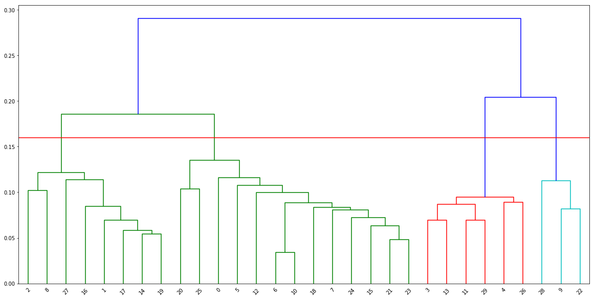
plt.axhline(y=0.16, color='r', linestyle='-')

plt.show()

4 clusters are chosen here.
newclusters=[]
group1=[2,8,27,16,1,17,14,19]
group2 = [20,25,0,5,12,6,10,18,7,24,15,21,23]
group3 = [3,13,11,29,4,26]
group4 = [28,9,22]

newclusters.append([['group0'],customers.index[group1].tolist()])
newclusters.append([['group1'],customers.index[group2].tolist()])
newclusters.append([['group2'],customers.index[group3].tolist()])
newclusters.append([['group3'],customers.index[group4].tolist()])
pd.DataFrame(np.array(newclusters))
| 0 | 1 | |
|---|---|---|
| 0 | [group0] | [Austin Cruisers, Indianapolis Velocipedes, Seattle Race Equipment, Nashville Cruisers, Ann Arbor Speed, New Orleans Velocipedes, Miami Race Equipment, Oklahoma City Race Equipment] |
| 1 | [group1] | [Philadelphia Bike Shop, San Antonio Bike Shop, Albuquerque Cycles, Dallas Cycles, Los Angeles Cycles, Denver Bike Shop, Kansas City 29ers, New York Cycles, Detroit Cycles, Providence Bi-peds, Minneapolis Bike Shop, Phoenix Bi-peds, Portland Bi-peds] |
| 2 | [group2] | [Cincinnati Speed, Louisville Race Equipment, Las Vegas Cycles, Wichita Speed, Columbus Race Equipment, San Francisco Cruisers] |
| 3 | [group3] | [Tampa 29ers, Ithaca Mountain Climbers, Pittsburgh Mountain Machines] |
above is new clustering grouping
below is previous clsutering grouping
Compared to the results from KMeans, it was found cluster 0 and 4 were combined.
above group0 –> below group 1
above group1 –> below group0+below group4
above group2 –> below group3
above group3 –> below group2
pd.DataFrame(customers.reset_index().groupby("group")["bikeshop.name"].unique())
| bikeshop.name | |
|---|---|
| group | |
| 0 | [Philadelphia Bike Shop, San Antonio Bike Shop] |
| 1 | [Ann Arbor Speed, Austin Cruisers, Indianapolis Velocipedes, Miami Race Equipment, Nashville Cruisers, New Orleans Velocipedes, Oklahoma City Race Equipment, Seattle Race Equipment] |
| 2 | [Ithaca Mountain Climbers, Pittsburgh Mountain Machines, Tampa 29ers] |
| 3 | [Cincinnati Speed, Columbus Race Equipment, Las Vegas Cycles, Louisville Race Equipment, San Francisco Cruisers, Wichita Speed] |
| 4 | [Albuquerque Cycles, Dallas Cycles, Denver Bike Shop, Detroit Cycles, Kansas City 29ers, Los Angeles Cycles, Minneapolis Bike Shop, New York Cycles, Phoenix Bi-peds, Portland Bi-peds, Providence Bi-peds] |
Cluster 0 and 4
Cluster 0 –> Features of bikes: relatively low price, mixed-type bikes and frames Cluster 4 –> Features of bikes: relatively low price, mixed-type bikes and Aluminum frames
Cluster 0 and 4 are very similary and they can be combined into big groups: relatively low price, mixed-type bikes and mixed-type frames.
In hierachical clustering, with different criteria to cut tree, the results can be different. Thus, in this sense, cluster 0 and cluster 4 can be combined because of high similarity/closeness.