Email campaign
Email campaign is a common used tool for marketing. In this project, I would evaluate the email campaign performance and think of ways to improve the efficiency by analytics. It can be referred by Take-home data science challenges.
The datasets are given to answer the following questions:
- What percentage of users opened the email and what percentage clicked on the link within the email?
- The VP of marketing thinks that it is stupid to send emails to a random subset and in a random way. Based on all the information you have about the emails that were sent, can you build a model to optimize in future email campaigns to maximize the probability of users clicking on the link inside the email?
- By how much do you think your model would improve click through rate ( defined as # of users who click on the link / total users who received the email). How would you test that? Did you find any interesting pattern on how the email campaign performed for different segments of users? Explain.
Import datasets
email_opened_table.csv listed the id of the emails that were opened at least once.
email_table.csv showcased the details of each email sent
link_clicked_table listed the id of the emails whose link inside was clicked at least once.
import os
import glob

files = [i for i in glob.glob('email/*.{}'.format('csv'))]
print(files)
['email\\email_opened_table.csv', 'email\\email_table.csv', 'email\\link_clicked_table.csv']
import pandas as pd

datasets={}
for file in files:
    datasets[file]=pd.read_csv(file)
openList  = datasets["email\\email_opened_table.csv"].email_id.tolist()
clickList = datasets['email\\link_clicked_table.csv'].email_id.tolist()

emails = datasets['email\\email_table.csv']
emails['open'] = emails.email_id.apply(lambda x: 1 if x in openList else 0)
emails['click'] = emails.email_id.apply(lambda x: 1 if x in clickList else 0)
emails.head()
| email_id | email_text | email_version | hour | weekday | user_country | user_past_purchases | open | click | |
|---|---|---|---|---|---|---|---|---|---|
| 0 | 85120 | short_email | personalized | 2 | Sunday | US | 5 | 0 | 0 |
| 1 | 966622 | long_email | personalized | 12 | Sunday | UK | 2 | 1 | 1 |
| 2 | 777221 | long_email | personalized | 11 | Wednesday | US | 2 | 0 | 0 |
| 3 | 493711 | short_email | generic | 6 | Monday | UK | 1 | 0 | 0 |
| 4 | 106887 | long_email | generic | 14 | Monday | US | 6 | 0 | 0 |
len(emails.email_id.unique())==len(emails.email_id)
True
Question 1
Percentage of opening and clicking
emails.open.mean()
0.10345
emails.click.mean()
0.021190000000000001
Question 2
build a model to optimize in future email campaigns to maximize the probability of users clicking
Exploratory Analysis
import matplotlib.pyplot as plt
import seaborn as sns

plt.figure(figsize=(10,5))
plt.title("length of email text vs click")
sns.countplot(emails.click,hue=emails.email_text)
<matplotlib.axes._subplots.AxesSubplot at 0x2058b02eeb8>
emails.groupby("email_text").click.mean().plot(kind="bar")
<matplotlib.axes._subplots.AxesSubplot at 0x20594b47f98>
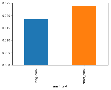
For users who clicks the email, short emails are more than long emails
plt.figure(figsize=(10,5))
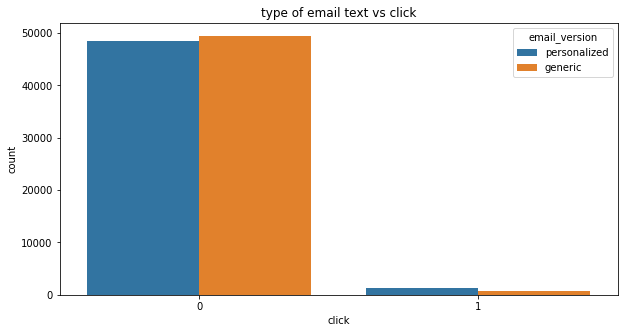
plt.title("type of email text vs click")
sns.countplot(emails.click,hue=emails.email_version)
<matplotlib.axes._subplots.AxesSubplot at 0x20595fd5f60>
emails.groupby("email_version").click.mean().plot(kind="bar")
<matplotlib.axes._subplots.AxesSubplot at 0x2058b07c198>
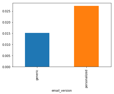
Personalized emails are more likely to be clicked
plt.figure(figsize=(10,5))
plt.title("Probability of clicking varies with hour")
emails.groupby("hour").click.mean().plot(kind="line")
<matplotlib.axes._subplots.AxesSubplot at 0x2058b15a4a8>
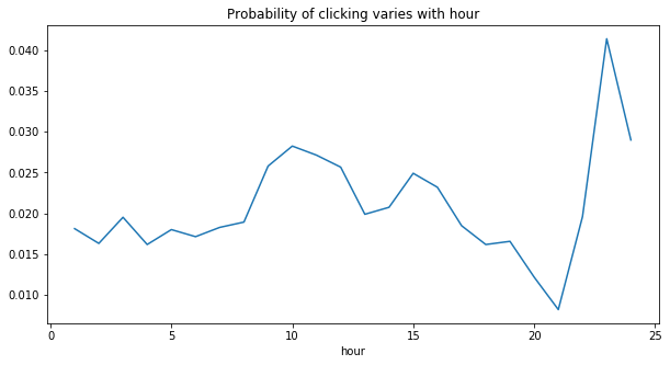
Two peaks for average clicking in 10 am and 23 pm
plt.figure(figsize=(10,5))
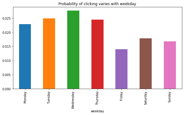
plt.title("Probability of clicking varies with weekday")
wdorder = [ 'Monday', 'Tuesday', 'Wednesday', 'Thursday', 'Friday', 'Saturday', 'Sunday']
emails.groupby("weekday").click.mean()[wdorder].plot(kind="bar")
<matplotlib.axes._subplots.AxesSubplot at 0x2058b1afbe0>
plt.figure(figsize=(10,5))
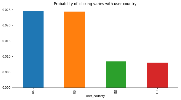
plt.title("Probability of clicking varies with user country")
emails.groupby("user_country").click.mean().sort_values(ascending=False).plot(kind="bar")
<matplotlib.axes._subplots.AxesSubplot at 0x2058b232710>
plt.figure(figsize=(10,5))
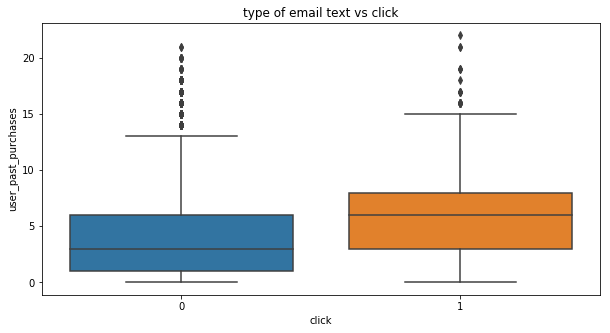
plt.title("type of email text vs click")
sns.boxplot(x=emails.click,y=emails.user_past_purchases)
<matplotlib.axes._subplots.AxesSubplot at 0x2058b2706d8>
Insights from visualization
A personalized email which is shorter sent to the loyal customers are more likely to be clicked
Time to build a model!
Modeling
100*(1-emails.click.mean())
97.881
emails.head()
| email_id | email_text | email_version | hour | weekday | user_country | user_past_purchases | open | click | |
|---|---|---|---|---|---|---|---|---|---|
| 0 | 85120 | short_email | personalized | 2 | Sunday | US | 5 | 0 | 0 |
| 1 | 966622 | long_email | personalized | 12 | Sunday | UK | 2 | 1 | 1 |
| 2 | 777221 | long_email | personalized | 11 | Wednesday | US | 2 | 0 | 0 |
| 3 | 493711 | short_email | generic | 6 | Monday | UK | 1 | 0 | 0 |
| 4 | 106887 | long_email | generic | 14 | Monday | US | 6 | 0 | 0 |
def decodeText(x):
    if x=="short_email":
        return 0
    if x=="long_email":
        return 1
    return x

def decodeVersion(x):
    if x=="personalized":
        return 1
    if x=="generic":
        return 0
    return x

def decodeHour(x):
    if x<=6 or x>=23:
        return "night"
    if x>=7 and x<=12:
        return "morning"
    if x<=18 and x>12:
        return "afternoon"
    if x<23 and x>18:
        return "evening"


emails['email_text'] = emails['email_text'].apply(decodeText)
emails['email_version'] = emails['email_version'].apply(decodeVersion)
emails['hour'] = emails['hour'].apply(decodeHour)
def decodeWeek(x):
    if x=="Sunday" or x=="Saturday":
        return 1
    else:
        return 0

emails['weekday']=emails.weekday.apply(decodeWeek)
emails.head()
| email_id | email_text | email_version | hour | weekday | user_country | user_past_purchases | open | click | |
|---|---|---|---|---|---|---|---|---|---|
| 0 | 85120 | 0 | 1 | night | 1 | US | 5 | 0 | 0 |
| 1 | 966622 | 1 | 1 | morning | 1 | UK | 2 | 1 | 1 |
| 2 | 777221 | 1 | 1 | morning | 0 | US | 2 | 0 | 0 |
| 3 | 493711 | 0 | 0 | night | 0 | UK | 1 | 0 | 0 |
| 4 | 106887 | 1 | 0 | afternoon | 0 | US | 6 | 0 | 0 |
X=pd.get_dummies(emails,columns=["hour","user_country"],drop_first=True).drop(["email_id",'open','click'],axis=1)
y=emails['click']
X.head()
| email_text | email_version | weekday | user_past_purchases | hour_evening | hour_morning | hour_night | user_country_FR | user_country_UK | user_country_US | |
|---|---|---|---|---|---|---|---|---|---|---|
| 0 | 0 | 1 | 1 | 5 | 0 | 0 | 1 | 0 | 0 | 1 |
| 1 | 1 | 1 | 1 | 2 | 0 | 1 | 0 | 0 | 1 | 0 |
| 2 | 1 | 1 | 0 | 2 | 0 | 1 | 0 | 0 | 0 | 1 |
| 3 | 0 | 0 | 0 | 1 | 0 | 0 | 1 | 0 | 1 | 0 |
| 4 | 1 | 0 | 0 | 6 | 0 | 0 | 0 | 0 | 0 | 1 |
Notice: the dataset is highly imbalanced
from sklearn.model_selection import train_test_split
from sklearn.linear_model import LogisticRegression
from sklearn.tree import DecisionTreeClassifier
from sklearn.ensemble import RandomForestClassifier
import xgboost as xgb

from sklearn.metrics import classification_report

X_train,X_test,y_train,y_test = train_test_split(X,y,test_size=0.3,random_state=42,stratify = y)
XGB for the first time
#model = LogisticRegression(class_weight="balanced")
#model = DecisionTreeClassifier(max_depth=30,max_features=10)
model = RandomForestClassifier(class_weight={1:60,0:1})
#model = xgb.XGBClassifier(objective='binary:logistic',n_estimors=10,seed=123,early_stopping_rounds=30,
 #                        eta=0.1,num_boost_round=30,scale_pos_weight=60)

model.fit(X_train,y_train)
y_pred = model.predict(X_test)

print(classification_report(y_test,y_pred))
             precision    recall  f1-score   support

          0       0.99      0.66      0.79     29364
          1       0.04      0.58      0.07       636

avg / total       0.97      0.66      0.78     30000
#model = LogisticRegression(class_weight="balanced")
#model = DecisionTreeClassifier(max_depth=30,max_features=10)
#model = RandomForestClassifier(class_weight={1:60,0:1})
model = xgb.XGBClassifier(objective='binary:logistic',n_estimors=10,seed=123,early_stopping_rounds=30,
                         eta=0.1,num_boost_round=30,scale_pos_weight=35)

model.fit(X_train,y_train)
y_pred = model.predict(X_test)

print(classification_report(y_test,y_pred))
             precision    recall  f1-score   support

          0       0.99      0.73      0.84     29364
          1       0.05      0.61      0.09       636

avg / total       0.97      0.73      0.82     30000
y_pred
array([ 0.01954367,  0.05587769,  0.02632774, ...,  0.01095612,
        0.01684568,  0.01666684], dtype=float32)
y_pred.sum()
8264
y_pred.sum()/len(y_pred)
0.27546666666666669
Old way will send out 30000 emails. New way will only send out to those who are predicted as “click”
The precision is 0.05, indicating the click-through rate is 5%, doubling the original rate 2%. Thus the model is good. It will cover 61% the clicked people.
Using this model, we can double the click-through rate with 28% emails. We can save resouces in the people who will not click.
Also, for the first time, I tried XGB and I will use it in future analyses.
Conclusion
To verify the exact effect of my model, A/B Testing can be used.
pd.Series(model.feature_importances_,index=X.columns).sort_values(ascending=False)
user_past_purchases    0.650852
email_version          0.072684
weekday                0.049924
email_text             0.043801
user_country_FR        0.042266
user_country_UK        0.037051
user_country_US        0.036576
hour_morning           0.026804
hour_night             0.025937
hour_evening           0.014105
dtype: float64
Appendix
Email campaigns for different segments
from sklearn.preprocessing import StandardScaler

users = X.drop(["email_version","weekday","email_text","hour_evening","hour_morning","hour_night"],axis=1)
X_std=StandardScaler().fit_transform(users)
from sklearn.cluster import KMeans

intertias=[]
for i in range(2,10):
    cluster = KMeans(n_clusters=i,random_state=42)
    cluster.fit(X_std)
    intertias.append(cluster.inertia_)
plt.figure(figsize=(10,5))
plt.title("Choose K")
plt.plot(range(2,10),intertias)
[<matplotlib.lines.Line2D at 0x2becf96ba58>]
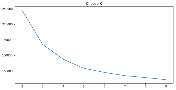
cluster = KMeans(n_clusters=3,random_state=42)
cluster.fit(X_std)
KMeans(algorithm='auto', copy_x=True, init='k-means++', max_iter=300,
    n_clusters=3, n_init=10, n_jobs=1, precompute_distances='auto',
    random_state=42, tol=0.0001, verbose=0)
pd.Series(y).groupby(cluster.labels_).mean()
0    0.024675
1    0.022079
2    0.008004
Name: click, dtype: float64
pd.Series(cluster.labels_).value_counts()
1    70066
0    19939
2     9995
dtype: int64
y.mean()
0.021190000000000001
users.groupby(cluster.labels_).mean()
| user_past_purchases | user_country_FR | user_country_UK | user_country_US | |
|---|---|---|---|---|
| 0 | 3.843673 | 0.0 | 1.0 | 0.000000 |
| 1 | 3.882140 | 0.0 | 0.0 | 0.857748 |
| 2 | 3.921961 | 1.0 | 0.0 | 0.000000 |
Insights:
If we segment customers according to their demographic info, we can find there are four groups. Two groups have relatively high click through rate. Since we only have two features, it is not a good clustering results.